Univariate Statistics
- Measure distribution of a single variable
- 4 types of measures:
- Central Tendency
- Dispersion
- Distribution Shape
- Graphical Representation
- Define “univariate”: analyze one variable at a time.
- Give 2–3 real-world examples (height, test score, income).
- State learning objective: summarize and interpret a single variable.
Central Tendencies
- Mean: Average of all values
- Median: Middle values when sorted
- Mode: Most frequent value
- Explain when to prefer each measure:
- Mean: use for symmetric data.
- Median: robust to outliers or skew.
- Mode: useful for categorical or multimodal data.
- Note median for even n = average of two middle values.
- Suggest quick demo comparing mean vs median with an outlier.
Dispersion
- Range: Difference between max and min
- Variance: Average of squared differences from mean
- Standard Deviation: Square root of variance
- Emphasize purpose: quantify spread beyond center.
- Range: simple but sensitive to outliers.
- Variance/SD: summarize spread around mean; SD returns to original units.
Variance
\[ s^2 = \frac{\sum_{i=1}^{n} (x_i - \bar{x})^2}{n-1} \]
- \(s^2\) is the sample variance
- \(n\) is the number of observations in the sample
- \(x_i\) is the \(i\)th observation in the sample
- \(\bar{x}\) is the sample mean
- Walk through formula: deviations, square, sum, divide by n-1.
- Explain Bessel’s correction (n-1) for unbiased estimation.
- Contrast with population variance (divide by N).
Variance Use
- Variance is used to measure how spread out the values in a data set are
- A high variance indicates that the data points are very spread out from the mean
- Interpret: larger variance = more spread.
- Limitation: units are squared, less intuitive than SD.
- Advice: compare variances only for same-scale variables.
Standard Deviation
\[ s = \sqrt{\frac{\sum_{i=1}^{n} (x_i - \bar{x})^2}{n-1}} \]
- \(s\) is the sample standard deviation
- \(n\) is the number of observations in the sample
- \(x_i\) is the \(i\)th observation in the sample
- \(\bar{x}\) is the sample mean
- SD = sqrt(variance); same units as data.
- Intuition: typical distance from the mean (summary metric).
- Mention sensitivity to outliers.
Standard Deviation Use
- Turns variance into a more understandable metric
- Standard deviation explains how much the data deviates from the mean
- Each standard deviation away from the mean accounts for a certain percentage of the data
- Introduce empirical rule (68/95/99.7) for approx. normal data.
- Warn: empirical rule assumes normality; may not hold if skewed.
- Suggest alternatives: IQR, MAD for non-normal data.
Distribution Shape
- Skewness: Measure of symmetry in data
- Kurtosis: Measure of the “tailedness” of the data
import pandas as pd
import numpy as np
import matplotlib.pyplot as plt

mean = 0
std = 1
sample_num = 1000
data = np.random.normal(mean, std, sample_num)
data = [round(x, 2) for x in data]
mode = pd.Series(data).mode()[0]
median = pd.Series(data).median()

plt.hist(data, bins=30, density=True, alpha=0.6, color="g")

xmin, xmax = plt.xlim()
x = np.linspace(xmin, xmax, 100)
p = np.exp(-0.5 * (x - mean) ** 2 / std**2) / (std * np.sqrt(2 * np.pi))

plt.plot(x, p, "k", linewidth=2)
title = "Gaussian Distribution\nMean = {:.2f}, Median = {:.2f}, Mode {:.2f}\nstd = {:.2f}".format(
    mean, median, mode, std
)

plt.axvline(mean, color="b", linestyle="dashed", linewidth=2, label="Mean")
plt.axvline(median, color="r", linestyle="dashed", linewidth=2, label="Median")
plt.axvline(mode, color="y", linestyle="dashed", linewidth=2, label="Mode")

plt.legend()

plt.title(title)
plt.xlabel("Value")
plt.ylabel("Frequency")

plt.show()
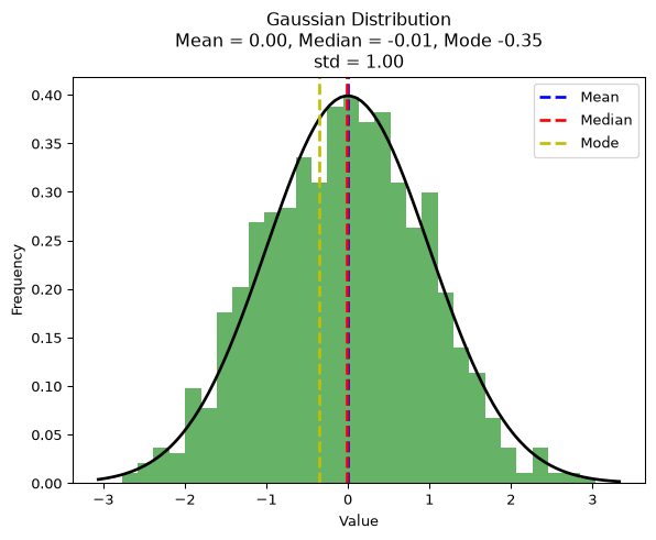
- Run code to show histogram + theoretical normal curve.
- Highlight vertical lines: mean (blue), median (red), mode (yellow).
- Demo ideas: change mean/std or sample size to show variability.
Skewness: Normal, Gaussian, Bell Curve
- 68% of data falls within 1 standard deviation
- 95% of data falls within 2 standard deviations
- 99.7% of data falls within 3 standard deviations
- Mean = Median = Mode
- Reinforce empirical rule and its normality assumption.
- Use to connect SD with probability mass for symmetric data.
- Note equality of mean/median/mode is a property of symmetry.
Skewness: Positive/Negative
- Positive Skewness: Tail is farther on the larger side of the x-axis
- Negative Skewness: Tail is farther on the smaller side of the x-axis
- Explain effect on mean vs median:
- Right-skew (positive): mean > median.
- Left-skew (negative): mean < median.
- Give examples of right-skewed data: income, wait times.
Kurtosis
- Measure of the “tailedness” of the data
- The more the Kurtosis, the more the data is in the tails
- Normal Distribution has a Kurtosis of 3
- Higher Kurtosis: More data in the tails
- Lower Kurtosis: Less data in the tails
- Measures how many outliers.
- Define kurtosis and “excess kurtosis” (kurtosis − 3).
- Interpret: high kurtosis → heavier tails → more extremes.
- Warn: kurtosis sensitive to a few outliers.