Num2Num Stats

Bivariate Statistics: Num 2 Num

Correlation

Wisdom

Age

Independent and Dependent Variables

  • Dependent variable
    • What you want to predict or explain
  • Independent variable
    • the variable that explains or predicts the outcome of the dependent variable.
  • Age = Independent variable
  • Wisdom = Dependent variable

Correlation Measurement

  • How much wisdom can be explained by age?

Pearson Correlation Coefficient: r

  • Measures the strength and direction of the linear relationship between two variables.
  • Ranges from -1 to 1
  • 0 means no correlation
  • 1 means perfect positive correlation
  • -1 means perfect negative correlation

Pearson coefficient formula

\[ r_{x,y} = \frac{\sum_{i=1}^{n} (X_i - \bar{X})(Y_i - \bar{Y})}{\sqrt{\sum_{i=1}^{n} (X_i - \bar{X})^2 \sum_{i=1}^{n} (Y_i - \bar{Y})^2}} \]

  • numerator: sum of the product of the differences between each pair of observations and the mean of each variable
  • denominator: square root of the product of the variance of each variable

Pearson Coefficient Output

  • Positive number means positive correlation
    • As the independent variable increases, the dependent variable also increases.
  • Negative number means negative correlation
    • As the independent variable increases, the dependent variable decreases.

Qualifications

  • Must be continuous data.
    • not ranked data, ordinal data, or categorical data
  • Must have Linear relationship
    • Will not detect variability that expands or contracts at different points.
  • Homoscedastic (equal variance)
    • The variability of the dependent variable is the same at all levels of the independent variable.

Skewness, Kurtosis and these assumptions

  • Skewness can indicate non-linearity
  • Kurtosis can indicate presence of outliers.

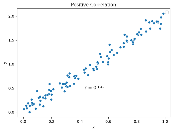
Example: Positively correlated

import seaborn as sns
import pandas as pd
import matplotlib.pyplot as plt
import numpy as np

np.random.seed(42)

# Generate positively correlated datasets
x1 = np.random.rand(100)
y1 = 2 * x1 + np.random.normal(0, 0.1, 100)
df1 = pd.DataFrame({'x': x1, 'y': y1})

a = sns.scatterplot(data=df1, x='x', y='y')
text = f"r = {df1.corr().loc['x', 'y']:.2f}"
plt.text(0.5, 0.5, text, fontsize=12, ha='center', va="center")
a.set_title('Positive Correlation')
a.legend()
plt.show()
/tmp/ipykernel_504852/1546156619.py:17: UserWarning: No artists with labels found to put in legend.  Note that artists whose label start with an underscore are ignored when legend() is called with no argument.
  a.legend()
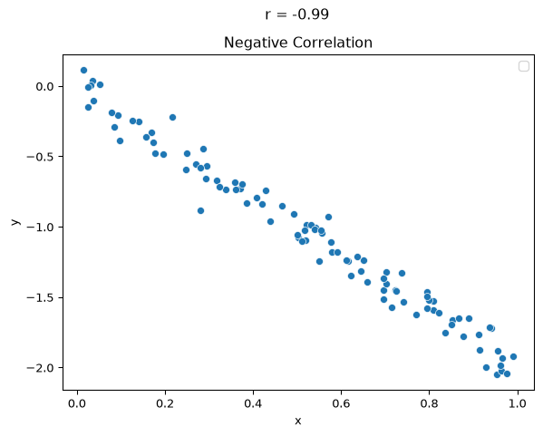
Example: Negatively correlated

import scipy.stats as stats

x2 = np.random.rand(100)
y2 = -2 * x2 + np.random.normal(0, 0.1, 100)
df2 = pd.DataFrame({"x": x2, "y": y2})

b = sns.scatterplot(data=df2, x="x", y="y")
b.set_title("Negative Correlation")
text = f"r = {df2.corr().loc['x', 'y']:.2f}"
b.text(0.5, 0.5, text, fontsize=12, ha="center", va="center")
b.legend(loc="upper right")
plt.show()
/tmp/ipykernel_504852/1827419204.py:11: UserWarning: No artists with labels found to put in legend.  Note that artists whose label start with an underscore are ignored when legend() is called with no argument.
  b.legend(loc="upper right")

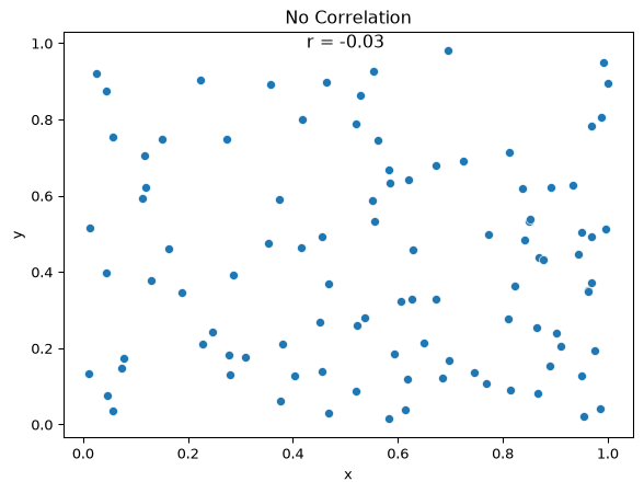
Example: No correlation

x3 = np.random.rand(100)
y3 = np.random.rand(100)
df3 = pd.DataFrame({"x": x3, "y": y3})

c = sns.scatterplot(
    data=df3, x="x", y="y"
)
text = f"r = {df3.corr().loc["x", "y"]:.2f}"
c.text(0.5, 1, text, fontsize=12, ha="center", va="center")
c.set_title("No Correlation")
plt.show()

Probability value

  • p-value
  • Measures probability that future data will return a 0.0 correlation.
  • p-value < 0.05 is typically considered significant.
  • p-value > 0.05 is typically considered not significant.
  • TL;DR: measures statistical significance of the correlation & lower == better.

Two ways to calculate

  • scipy.stats.pearsonr(x, y)
    • includes p-value
  • df.corr(numeric_only=True)
    • does not include p-value

Example: df.corr()

import pandas as pd

url = "https://raw.githubusercontent.com/dataprofessor/data/refs/heads/master/penguins_cleaned.csv"

df = pd.read_csv(url)
df.corr(numeric_only=True)
bill_length_mm bill_depth_mm flipper_length_mm body_mass_g
bill_length_mm 1.000000 -0.228626 0.653096 0.589451
bill_depth_mm -0.228626 1.000000 -0.577792 -0.472016
flipper_length_mm 0.653096 -0.577792 1.000000 0.872979
body_mass_g 0.589451 -0.472016 0.872979 1.000000

Example: scipy.stats.pearsonr()

import pandas as pd
import scipy.stats as stats

url = "https://raw.githubusercontent.com/dataprofessor/data/refs/heads/master/penguins_cleaned.csv"

df = pd.read_csv(url)
stats.pearsonr(df["bill_length_mm"], df["body_mass_g"])
PearsonRResult(statistic=np.float64(0.5894511101769491), pvalue=np.float64(1.538613514485931e-32))
r, p = stats.pearsonr(df["bill_length_mm"], df["body_mass_g"])
print(f"r: {round(r, 4)}, p: {round(p, 6)}")
r: 0.5895, p: 0.0